Satellite Data Science in Python
Sentinel-2 from scratch in pure Python
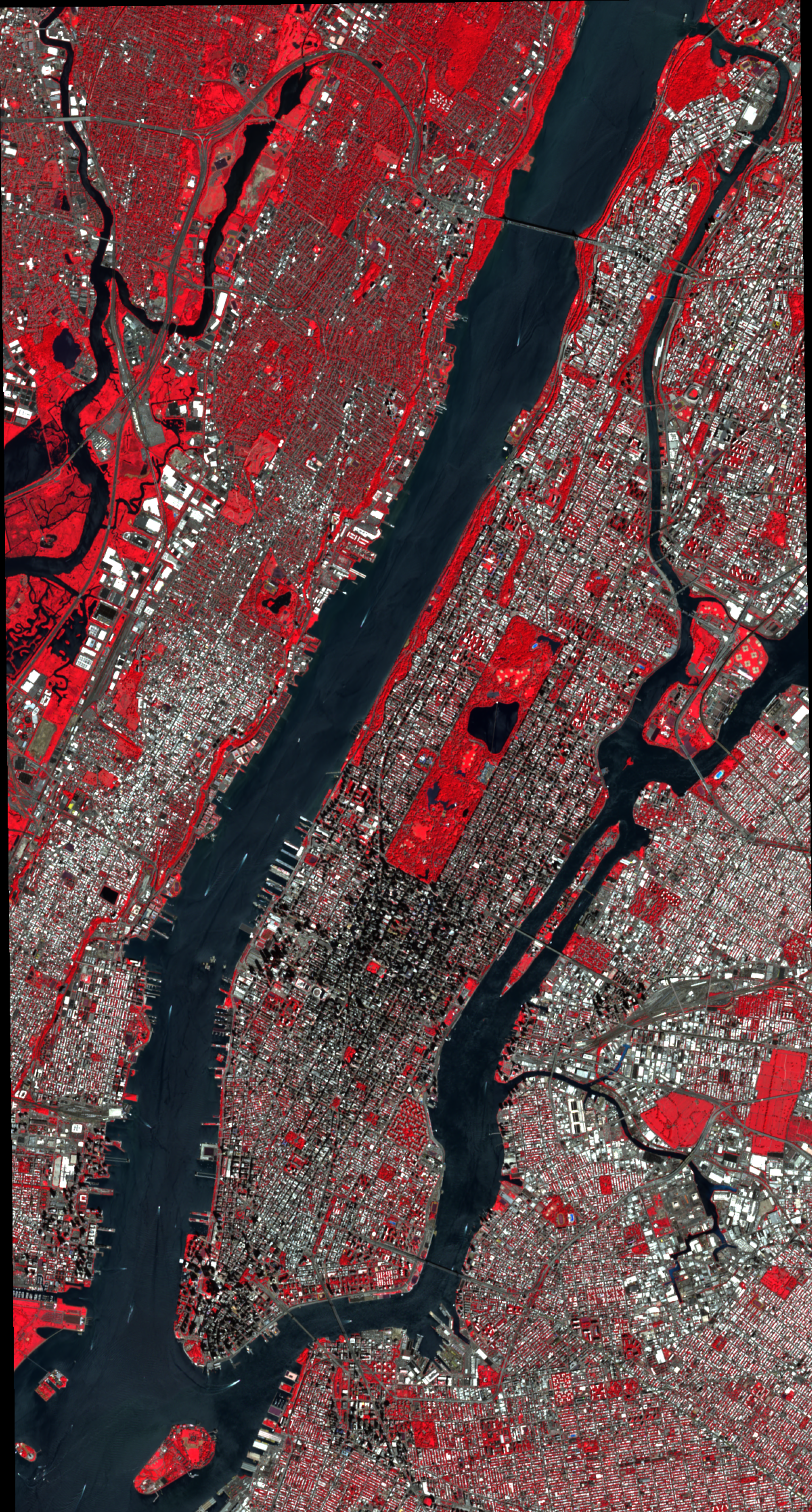
Open the satellite archive yourself — no platform, no account, no Earth Engine.
Satellites measure every point on Earth every few days, and the data is free. Almost nobody uses it, because the usual on-ramp is a platform that hides the measurement behind a login and a query language. This course takes the other route: you build the pipeline yourself, in pure Python, on a normal laptop — from a raster you draw by hand to a land-cover map of Manhattan you trained. Five chapters, one city, and every result interpreted with its limitation stated out loud.
WHAT YOU'LL BUILD
You don't call a platform API and accept what comes back. You acquire the imagery, correct it, and reason about it yourself.
A raster from first principles. A 64×64 array becomes a georeferenced GeoTIFF the moment you give it an affine transform and a CRS. You see the same array in index space and in map space, and understand exactly what the transform buys you — before a single byte of real imagery is downloaded.
A real Sentinel-2 acquisition pipeline. Search a public STAC catalog by place, date and cloud cover, choose a scene deterministically, and pull only the bands you need, cropped to your area. Convert raw integers to physical surface reflectance, handle the +1,000 BOA offset by reading the catalog flag rather than guessing, and save a four-band stack every later chapter reads.
Three spectral indices, built as separators. NDVI, NDWI and NDBI from one arithmetic recipe, tested on three patches of Manhattan that could not differ more — the built core, Central Park's canopy, and the Lake. Then every pixel becomes a seven-number feature vector: the exact form a classifier consumes.
A two-year data cube. Median composites reduce many cloudy scenes into one clean frame per quarter. Stack the quarters and read the cube two ways — as a filmstrip of the city greening and fading, and as curves where the park arches through the seasons while the built core and the Hudson stay flat as honest controls. Then a change map, and a green-up map dating when each place turns green.
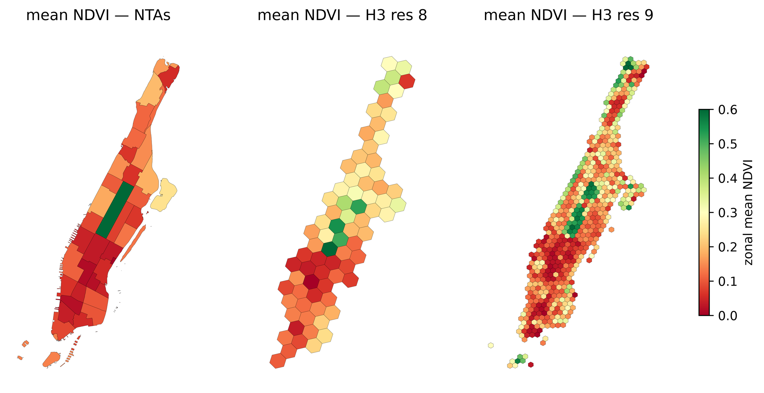
Green space per capita. Neighbourhood polygons from New York's open data API, weighed against H3 hexagons as a neutral alternative, with population from the global GHSL grid — acquired the deliberately awkward way, in World Mollweide, because real data arrives in the producer's CRS. Zonal statistics turn pixels into places, and green square metres per person turns places into a question about equality.
A land-cover map of Manhattan. OpenStreetMap supplies the labels, Chapter 2's indices supply the features. A transparent KNN first, then a random forest on identical input. Then you add roads as a fourth class specifically to watch it fail at 10 m — because a sensor telling you its limit is a result, not a defeat.
WHO THIS IS FOR
You work in GIS and have used Earth Engine or a commercial platform, but couldn't say what happens between "raw scene" and "NDVI layer" — and it bothers you.
You're a data scientist moving into spatial problems and need imagery to stop being an opaque blob and start being an array with known units.
You work in urban planning, environment, agriculture or real estate and want to produce your own vegetation, seasonality and land-cover maps rather than commissioning them.
You've been blocked from remote sensing by signup walls, quotas and API keys, and want a path that needs none of them.
You're heading toward deep learning on imagery and need the foundation those models assume: clean, correct, well-understood rasters.
WHAT YOU'LL LEARN
By the end of this course you can:
Explain what makes an array a raster — the transform and the CRS — and read, write and reproject georeferenced data with rasterio without guessing.
Search a public satellite archive by place, time and cloud cover, and download exactly the bands you need, cropped, with no account and no API key.
Convert raw digital numbers into surface reflectance correctly, including the processing-baseline offset that silently breaks cross-scene comparison when handled wrong.
Say precisely what scene-level cloud cover does and does not tell you, and build a real per-pixel cloud or class mask from the Scene Classification Layer.
Compute NDVI, NDWI and NDBI from first principles, prove they separate using distributions rather than pretty maps, and know why NDBI inherits a resolution compromise the others don't.
Build a multi-year time series from cloudy scenes using median composites, and read the resulting data cube as both imagery and signal.
Distinguish seasonality from real land-cover change — and know why comparing summer to winter mostly measures the deciduous cycle.
Aggregate pixels into places with zonal statistics, and defend your choice of spatial unit against the modifiable areal unit problem instead of ignoring it.
Resample data correctly by knowing what it represents — why interpolating reflectance is right and interpolating a population count invents people.
Train and evaluate a per-pixel land-cover classifier from open labels, and read its output up close, including where and why it fails.
COURSE STRUCTURE
Chapter 0 — Setting Up Your Satellite Environment. One conda command builds the environment for the whole course. Verification cells confirm every dependency and that your network can reach the public catalog.
Chapter 1 — Rasters & Real Sentinel-2 Data. Build a raster by hand, then a real one: STAC search, cropped download, reflectance conversion, composites, masking with polygons and classes, and an interactive map to check it lands where it should.
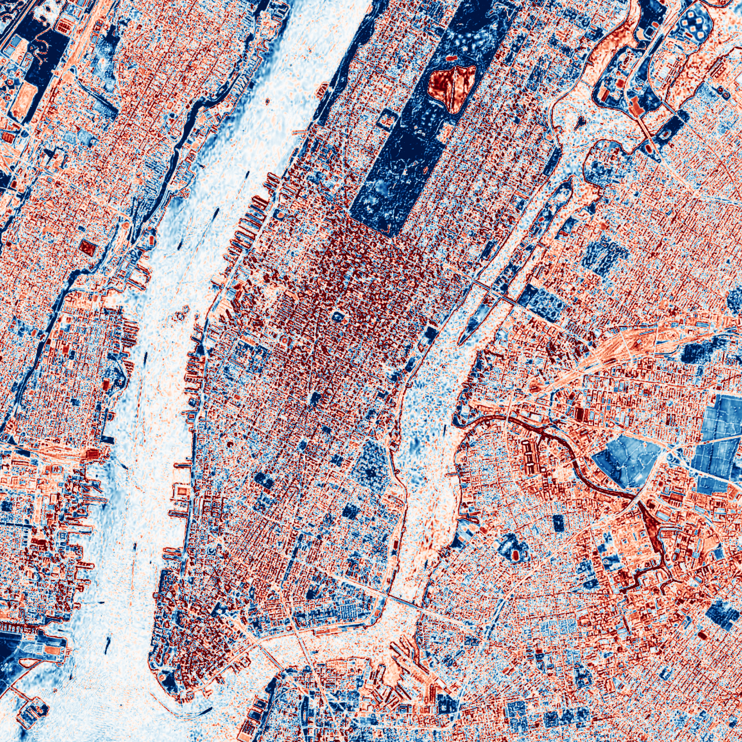
Chapter 2 — The Core Satellite Indices. One recipe, three indices, three test patches. Distributions prove separation, and every pixel ends as a seven-number feature vector.
Chapter 3 — The Temporal Dimension. Median composites, a two-year quarterly data cube, filmstrip and curves, change between two dates, and a green-up map — with the caveats that come with each.
Chapter 4 — Green Space Per Capita. Neighbourhoods against H3, population from GHSL in Mollweide, the count-resampling trap, and zonal features that answer a real per-person question.
Chapter 5 — Land-Cover Classification. OSM labels, KNN, random forest, a Bryant Park close-up, and an honest failure at 10 m.
WHAT'S INCLUDED
🎬 ~2.5 hours of video lectures on the New Science of Maps platform
📓 6 executed, self-contained notebooks (Chapters 0–5)
🛰️ Real Sentinel-2, GHSL and OpenStreetMap data — all free, all acquired in-course
♾️ Lifetime access, including future updates
PREREQUISITES / WHO IT'S NOT FOR
Prerequisites: comfortable Python and basic NumPy array thinking. No remote-sensing background needed — rasters, bands, CRS and reflectance are all built from first principles. No account, no API key, no paid data, and nothing that needs more than a normal laptop.
Recommended companions: for the geospatial Python foundations, see the book Geospatial Data Science Essentials: 101 Practical Python Tips and Tricks.
Next steps: GeoAI and urban analytics
INSTRUCTOR
Taught by Milan Janosov — geospatial data scientist, network scientist (PhD), and practitioner. You build alongside a working scientist, on real data, with honest attention to what each method can and can't tell you.